Velocity time graph – Comprehensive Guide

Last updated on February 8th, 2024 at 12:59 pm

The velocity-time graph is defined as a graphical representation of the velocity of a body in motion with respect to time.

Generally, velocity is assigned to the y-axis, and time is pointed to the x-axis.
This graph type is also written as a v-t graph or velocity-time graph.

The diagram below depicts a few velocity-time graphs, each depicting a specific type of linear motion.

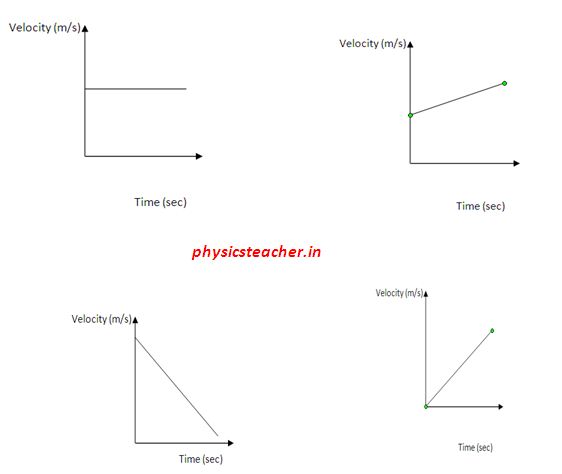
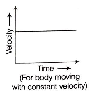
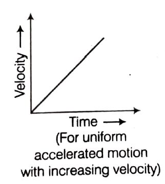
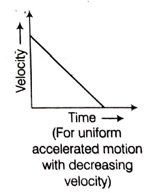
Velocity-time graph for motion with constant velocity

Velocity-time graph for motion with uniform acceleration

Velocity-time graph for motion with uniform retardation

Velocity-time graph for non-uniform acceleration & retardation

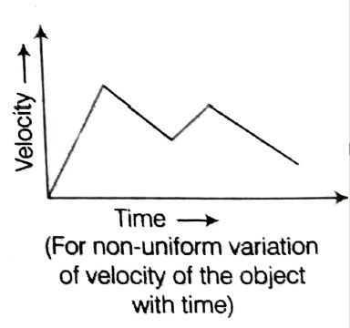
As we practically travel in linear motion, sometimes we have a uniform velocity, and sometimes we just accelerate for a duration. And again we slow down through retardation.

Here in this post, we will explain a case study of this kind of motion. The velocity-time graph presented here with the case study shows you all these kinds of scenarios.

Velocity Time Graph – Case Study with numerical calculation

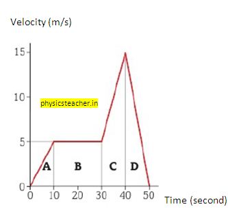
From the above v-t graph, find out the distance traveled in each section A, B, C, and D.
Also, find out the total distance traveled.

Explanation – section A

During this period velocity has changed from zero to 5 m/s.
And this change happened in a time duration of 10 seconds. That means the object in motion had an accelerated motion during this period.

From the equation of acceleration we get acceleration for section A = (v-u)/t = (5-0)/10 = 0.5 m/s²

[ t = time duration of a period = time at end of a period(t2) – time at the beginning of that period (t1) ]

The distance traversed in this period A = S1
= ut + ½ a t^2
S1 = 0 + ½ .0.5. 10^2=25 meter

---

Explanation – section B

Here, you can see that the velocity didn’t change at all and stayed at 5 m/s for the duration of (30-10) sec = 20 seconds.

So for a duration of 20 seconds of period B, the object had a uniform motion with a velocity of 5 m/s.

Now the distance traversed in this period B = S2 = v t = 5.20 m=100 m

---

Explanation – section C

In section C the object had again accelerated and changed its velocity from 5 m/s to 15m/s. And the time taken to make this velocity rise is = (40-30) s=10 seconds. we get the value of acceleration as =(v-u)/t =(15-5)/10 = 1 m/s^2

We can calculate the distance travelled during this period = S3.
S3 = ut + ½ a t^2 = 5.10 + 1/2 . 1.10^2 = 100 m

---

---

Explanation – section D

In this section we find the object slowing down to zero from a velocity of 15 m/s. And for this, it took a time duration of = (50-40)sec=10 seconds again.

The retardation during this period is = (0-15)/10= – 1.5 m/s^2. (note the negative sign)

The distance travelled in this period is = S4
S4 = ut + ½ a t^2 = 15.10 – 1/2 . 1.5.10^2 = 75 m

---

Case study (sections A, B, C, D) – summary

Along the path, the velocity has changed from zero to 5 m/s, then 15 m/s, and then again back to zero.

The body has experienced different values of acceleration, even had uniform motion and retardation.

The total distance travelled in 4 sections = (25+100+100+75)m = 300 meters.

---

Displacement from Velocity Time Graph

In the absence of a position-versus-time graph, a velocity-versus-time graph provides useful information about the change in the position, or displacement, of an object.

When an object travels with a constant velocity, it is obvious that the displacement of the object is equal to the area under a velocity-versus-time graph of its motion.

However, it is not so obvious when the motion is not constant. The graphs below describe the motion of an object that has an increasing velocity.

The motion of the object can be approximated by dividing it into time intervals of Δt and assuming that the velocity during each time interval is constant.

The approximate displacement during each time interval is equal to s = V_av t which is the same as the area under each rectangle. The approximate total displacement is therefore equal to the total area of the rectangles.

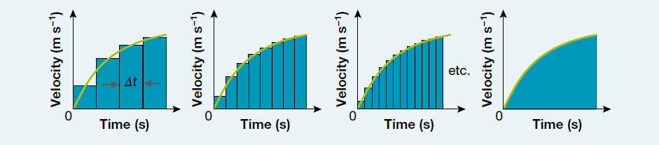
To better approximate the displacement, the graph can be divided into smaller time intervals. The total area of the rectangles is approximately equal to the displacement.

By dividing the graph into even smaller time intervals, even better estimates of the displacement can be made.

In fact, by continuing the process of dividing the graph into smaller and smaller time intervals, it can be seen that the displacement is, in fact, equal to the area under the graph.