Gauss’ Law – statement & derivation of equation

Last updated on June 19th, 2022 at 02:13 pm

Gauss’ law was formulated by the German mathematician and physicist Carl Friedrich Gauss (1777–1855). In presenting Gauss’ law, it will be necessary to introduce a new idea called electric flux.

The idea of flux involves both the electric field and the surface through which it passes. By bringing together the electric field and the surface through which it passes, we will be able to define electric flux and then present Gauss’ law. We will derive its equation as well for point charge within a spherical surface. And then we will derive the Gauss’ law equation for an arbitrarily shaped Gaussian surface also.

Derivation of Gauss’ law that applies only to a point charge

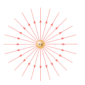
We begin by developing a version of Gauss’ law that applies only to a point charge, which we assume to be positive. The electric field lines for a positive point charge radiate outward in all directions from the charge, as shown in figure 1.

The magnitude E of the electric field at a distance r from the charge +q is E = kq/r².
The constant k can be expressed as k = 1/(4𝜋𝜀₀), where 𝜀₀ is the permittivity of free space.

With this substitution, the magnitude of the electric field becomes E = q/(4𝜋𝜀₀ r² ).

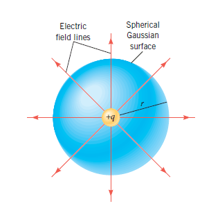
We now place this positive point charge at the center of an imaginary spherical surface of radius r, as Figure 2 shows. Such a hypothetical closed surface is called a Gaussian surface, although in general, it need not be spherical.

In figure 2, the electric field is perpendicular to the surface and has the same magnitude everywhere on it.

The surface area A of a sphere is A = 4𝜋 r², and the magnitude of the electric field can be written in terms of this area as
E = q/(A𝜀₀),
or EA = q / 𝜀₀ (when the electric field is perpendicular to the surface) ……… (1)

When the electric field is perpendicular to the surface, Gauss’ law for a point charge can be expressed primarily as EA = q / 𝜀₀, where the left side of Equation 1 is the product of the magnitude E of the electric field at any point on the Gaussian surface and the area A of the surface.

In Gauss’ law, this product is especially important and is called the electric flux, Φ_E and we can write Φ_E = E . A = EA cos θ

In other words, the electric flux Φ_E is defined as the scalar product of A and E. Hence, Φ_E = E . A = EA cos θ

Here, θ = angle between the electric field E and the area vector A. Note that the area vector is normal to the surface.

This means that when the electric field is perpendicular to the surface, it becomes parallel to the area vector. Thus, in this case, θ = 0°.
As, θ =0°. Hence, Φ_E = EA cos 0 = EA ………….(2)

Using equations (1) and (2) we now can write the equation of electric flux for a point charge: Φ_E = q / 𝜀₀

Gauss’ law for a point charge can be finally expressed as Φ_E = q / 𝜀₀ ………………… (3)

Gauss’ law states that the net electric flux through a closed Gaussian surface is equal to the total charge q inside the surface divided by ε₀.

This result indicates that, aside from the constant 𝜀₀, the electric flux Φ_E depends only on the charge q within the Gaussian surface and is independent of the radius r of the surface.

We will now see how to generalize Equation 2 to account for distributions of charges and Gaussian surfaces with arbitrary shapes.

Gauss’ law for an arbitrarily shaped Gaussian surface – derivation

Figure 3 shows a charge distribution whose net charge is labeled Q. The charge distribution is surrounded by a Gaussian surface—that is, an imaginary closed surface.

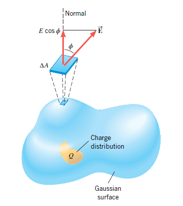
The surface can have any arbitrary shape (it need not be spherical), but it must be closed (an open surface would be like that of half an eggshell). The direction of the electric field is not necessarily perpendicular to the Gaussian surface. Furthermore, the magnitude of the electric field need not be constant on the surface but can vary from point to point.

To determine the electric flux through such a surface, we divide the surface into many tiny sections with areas ΔA1, ΔA2, and so on. Each section is so small that it is essentially flat and the electric field E is a constant (both in magnitude and direction) over it.

For reference, a dashed line called the “normal” is drawn perpendicular to each section on the outside of the surface.
To determine the electric flux for each of the sections, we use only the component of E that is perpendicular to the surface – that is, the component of the electric field that passes through the surface.

From Figure 3 it can be seen that this component has a magnitude of E cos ϕ, where ϕ is the angle between the electric field and the normal. The electric flux through any one section is then (E cos ϕ)ΔA.

The electric flux ΦE that passes through the entire Gaussian surface is the sum of all of these individual fluxes:
Φ_E = (E1 cos ϕ1)ΔA1 + (E2 cos ϕ2)ΔA2 + . . ., or
Φ_E = Σ(E cos ϕ)ΔA, where, as usual, the symbol Σ means “the sum of.”

Gauss’ law relates the electric flux Φ_E to the net charge Q enclosed by the arbitrarily shaped Gaussian surface.

GAUSS’ LAW
The electric flux Φ_E through a Gaussian surface is equal to the net charge Q enclosed by the surface divided by 𝜀₀, the permittivity of free space:
Φ_E = Σ(E cos ϕ)ΔA = Q/𝜀₀ …………….(3)

SI Unit of Electric Flux: N · m^2/C

Although we arrived at Gauss’ law by assuming the net charge Q was positive, Equation 3 also applies when Q is negative. In this case, the electric flux Φ_E is also negative. Gauss’ law is often used to find the magnitude of the electric field produced by a distribution of charges. The law is most useful when the distribution is uniform and symmetrical.