Simple Harmonic Motion (S.H.M) revision notes

Last updated on November 14th, 2021 at 04:09 pm

Simple harmonic motion is a type of periodic motion where the restoring force is directly proportional to the displacement (i.e., it follows Hooke’s Law). There are many situations where we can observe the special kind of oscillations called simple harmonic motion (s.h.m.).

---

Examples of Simple Harmonic Motion (S.H.M)

For example, the vibrating strings of a musical instrument show s.h.m. When plucked or bowed, the strings move back and forth about the equilibrium position of their oscillation.

In addition, other phenomena can be approximated by simple harmonic motion, such as the oscillation of spring, the motion of a simple pendulum, or molecular vibration.

A system that follows simple harmonic motion is known as a simple harmonic oscillator.

Here are some other situations where simple harmonic motion can be found:

• When a pure (single tone) sound wave travels through air, the molecules of the air vibrate with s.h.m.
• When an alternating current flows in a wire, the electrons in the wire vibrate with s.h.m.
• There is a small alternating electric current in a radio or television aerial when it is tuned to a signal in the form of electrons moving with s.h.m.

The requirements or conditions of Simple Harmonic Motion (S.H.M)

If a simple pendulum is undisturbed, it is in equilibrium.

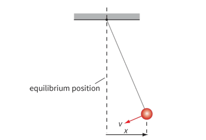
The string and the mass will hang vertically. To start the pendulum swinging (Figure 1), the mass must be pulled to one side of its equilibrium position.

The forces on the mass are unbalanced and so it moves back towards its equilibrium position.

The mass swings past this point and continues until it comes to rest momentarily at the other side; the process is then repeated in the opposite direction.

Note that a complete oscillation in Figure 1 is from right to left and back again.

The three requirements for S.H.M. of a mechanical system are:

• a mass that oscillates
• a position where the mass is in equilibrium
• a restoring force that acts to return the mass to its equilibrium position; the restoring force F is directly proportional to the displacement x of the mass from its equilibrium position and is directed towards that point.

The changes of velocity in s.h.m.

As the pendulum swings back and forth, its velocity is constantly changing.

• As it swings from right to left (as shown in Figure 1a above) its velocity is negative.
• It accelerates towards the equilibrium position and then decelerates as it approaches the other end of the oscillation.
• It has positive velocity as it swings back from left to right.
• Again, it has maximum speed as it travels through the equilibrium position and decelerates as it swings up to its starting position.
• This pattern of acceleration, followed by deceleration, changing direction, and acceleration again is characteristic of simple harmonic motion.

SHM Graphs ( graphs of displacement, velocity, and acceleration against time )

Idealized graphs of displacement, velocity, and acceleration against time are shown in Figure 2.

We will examine these graphs in sequence to see what they tell us about s.h.m. and how the three graphs are related to one another.

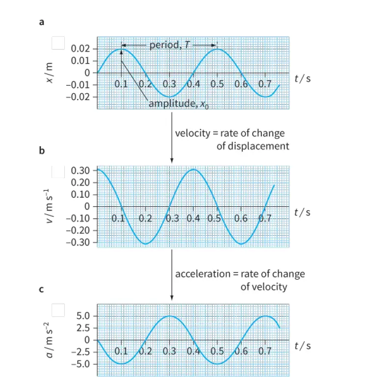
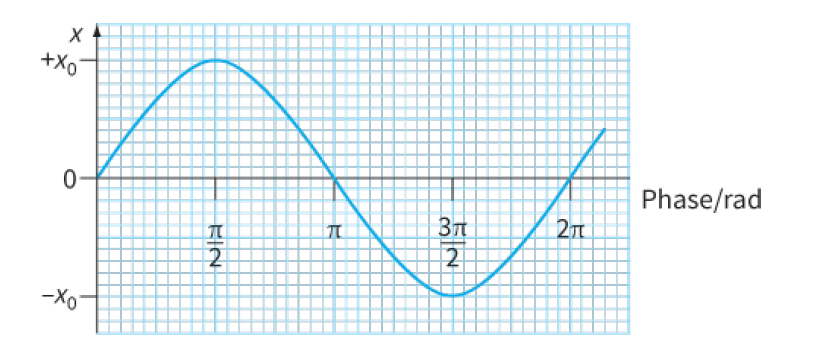
Displacement-time (x-t) graph

The displacement of the oscillating mass varies according to the smooth curve shown in Figure 2a.
Mathematically, this is a sine curve; its variation is described as sinusoidal.

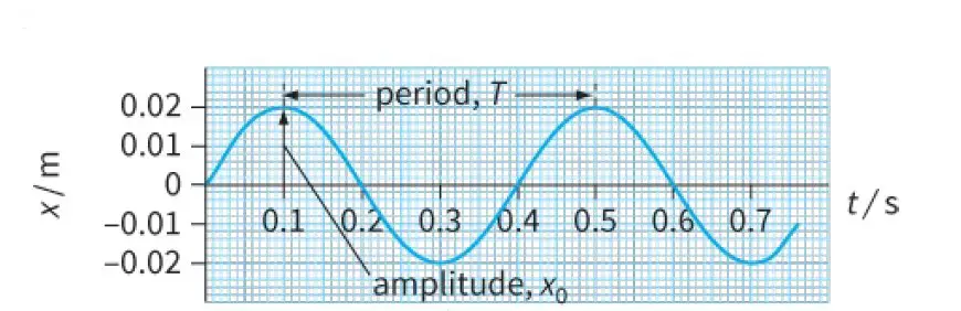
Note that this graph allows us to determine the amplitude x₀ and the period T of the oscillations.

In this graph, the displacement x of the oscillation is shown as zero at the start, when t is zero.

Note: We have chosen to consider the motion to start when the mass is at the midpoint of its oscillation (equilibrium position) and is moving to the right. We could have chosen any other point in the cycle as the starting point, but it is conventional to start as
shown here.

Velocity-time (v-t) graph

The velocity v of the oscillator at any time can be determined from the gradient of the displacement–time graph:
Again, we have a smooth curve (Figure 2b), which shows how the velocity v depends on time t.

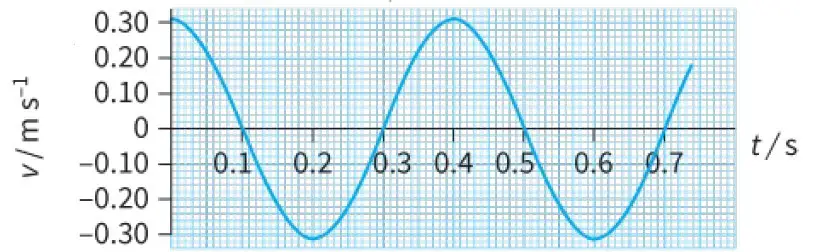
The shape of the curve is the same as for the displacement–time graph, but it starts at a different point in the cycle.

When time t = 0, the mass is at the equilibrium position and this is where it is moving fastest. Hence, the velocity has its maximum value at this point. Its value is positive because at time t = 0 it is moving towards the right.

Acceleration-time (a-t) graph

Finally, the acceleration a of the oscillator at any time can be determined from the gradient of the velocity-time graph:
This gives a third curve of the same general form (Figure 2c), which shows how the acceleration depends on time t.

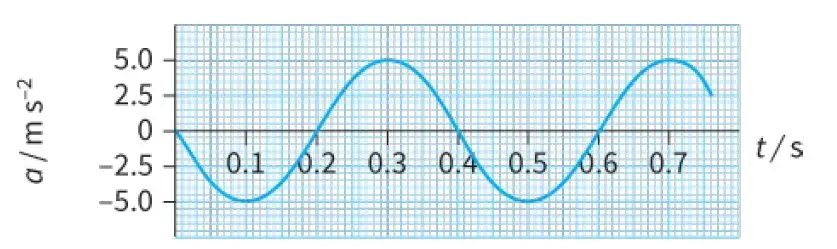
At the start of the oscillation, the mass is at its equilibrium position. There is no resultant force acting on it so its acceleration is zero.

As it moves to the right, the restoring force acts towards the left, giving it a negative acceleration.

The acceleration has its greatest value when the mass is displaced farthest from the equilibrium position.

Notice that the acceleration graph is ‘upside-down’ compared with the displacement graph. This shows that:

acceleration ∝ −displacement
or
a ∝ − x
In other words, whenever the mass has a positive displacement (to the right), its acceleration is to the left, and vice versa.

Frequency and angular frequency of s.h.m

The frequency f of s.h.m. is equal to the number of oscillations per unit time.

As we saw earlier, f is related to the time period T by this equation: f = 1/T

We can think of a complete oscillation of an oscillator or a cycle of s.h.m. as being represented by 2π radians.

This means, the phase of the oscillation changes by 2π rad during one oscillation.

Hence, if there are f oscillations in unit time, there must be 2πf radians in unit time.

This quantity is the angular frequency of the s.h.m. and it is represented by the Greek letter ω (omega).
The angular frequency ω is related to frequency f by the equation: ω = 2πf

Relationship of angular frequency ω to frequency f
ω = 2πf

Since, f = 1/T, the angular frequency ω is related to the period T of the oscillator by the equation:
ω = 2πf = ω = 2π/T
or, T = 2π/ω

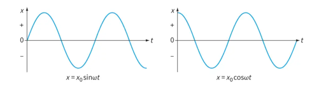
Equations of s.h.m.

The Displacement-time graph of an oscillator during s.h.m. is a sine curve.

We can present the same information in the form of an equation. The relationship between the displacement x and the time t is as follows:
x = x₀ sin ωt
where x₀ is the amplitude of the motion and ω is its frequency.

Sometimes, the same motion is represented using a cosine function, rather than a sine function:
x = x₀ cos ωt

Equations of simple harmonic motion:
x = x₀ sin ωt
x = x₀ cos ωt

The difference between these two equations is illustrated in Figure 4. The sine version starts at x = 0; that is, the oscillating mass is at its equilibrium position when t = 0.
The cosine version starts at x = x₀, so that the mass is at its maximum displacement when t = 0.
Note that, in calculations using these equations, the quantity ωt is in radians.